We've seen that phylogenetic tree algorithms can construct many different "good" putative evolutionary histories. An important and challenging problem is that of reducing a large number of trees to a smaller number of representative solutions. The objective of this assignment is to explore techniques for dealing with large sets of different phylogenetic trees for the same data. This assignment is inspired by the paper Statistically based postprocessing of phylogenetic analysis by clustering by Cara Stockham, Li-San Wang, and Tandy Warnow (Bioinformatics, Vol 18, Suppl. 1, 2002, pp. S285-S293).
In Part 1, you will implement the Robinson-Foulds distance metric. In Part 2, you will use a clustering algorithm to partition distinct phylogenetic trees into clusters of trees where the trees in a given cluster are similar with respect to Robinson-Foulds distance. In Part 3, you'll implement a general consensus algorithm that will allow you to find a consensus tree for each cluster and measure the quality of the cluster by its "specificity" - how close it is to being a binary tree.
Throughout this problem, We assume here that trees are binary but unrooted. So, the leaves have degree 1 (that is, 1 neighbor) and the internal nodes all have degree 3.
We use a version of the standard Newick format to represent trees. If a tree was rooted, you can imagine representing it as an ordered pair (A, B) where A is the left subtree, B is the right subtree, and there is an implicit root joining them. We use this same format for our unrooted trees as follows. First, for the main tree, the left subtree is a leaf and we make sure that all trees in our file have that same leaf as their left subtree. That's our "special" leaf. The root of the main tree shouldn't really be there, since an unrooted tree has no internal nodes of degree 2. So, we remove that root and replace its two edges by a single edge connecting the left subtree to the right subtree.
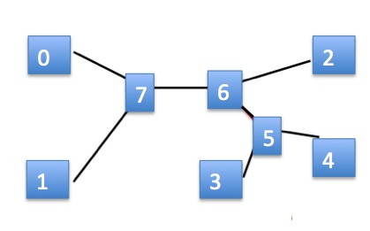
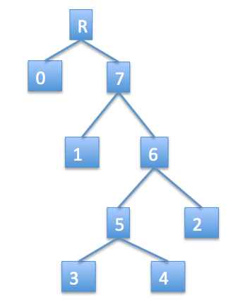
Consider the unrooted tree of interest below left and let leaf 0 be our special leaf. Then the rooted tree would be on the right, with a new dummy root inserted at the top. We represent our unrooted tree as if it were the rooted tree, but with the implicit understanding that the dummy root is missing and instead there is an edge between vertices 0 and 7. Of course, we only explicitly write the leaves in this representation, so the internal nodes are impliclit. The representation in tuple form would be:
(0, (1, ((3, 4), 2)))
Since order of subtrees doesn't matter, there are several other ways that this tree could be represented (by simply switch left and right subtrees wherever we wish).


Recall from class that the Robinson-Foulds distance between two trees is defined as follows: Given two trees T1 and T2 on the same set of leaves, consider each edge of T1. It's removal induces a partition of the leaves. That is, the removal of the edge results in a set S of leaves that remain connected to one another and another set R of leaves that are connected to one another, but the two sets are disconnected. If the removal of some edge of T2 induces the same partition, then this partition is not unique to T1. However, if no edge of T2 induces the same partition, this edge is unique to T1. We add up the number of partitions that are unique to T1 and, analogously, the number of partitions that are unique to T2 (that is, edges of T2 that induce a partition such that no edge in T1 induces the same partition). The Robinson-Foulds distance between T1 and T2 is equal to one half of the total number of unique partitions.
Under the assumption that the two trees have exactly the same leaves (and you can make this assumption here) we can do something slightly simpler: We can just find the number of partitions that are unique to T1! The number of partitions that are unique to T2 will be the same, so we don't need to compute that. (Sometimes, Robinson-Foulds is applied to trees that differ in their leaves, which is why we compute in both directions and then multiply the sum by 1/2. However, you should assume here that the two trees will always have the same leaves.)
As we noted in class, the "obvious" algorithm for computing the Robinson-Foulds distance takes O(N3) time. The fast randomized algorithm for computing the distance between trees T1 and T2 works in O(N) time as follows:
Your job is to implement this algorithm in a function called distance(Tree1, Tree2). The details of how to implement this are up to you, but you must use the fast O(N) approach described above, including using the efficient built-in integer xor.
Here is some test data. The distance between the two trees T1 and T2 below is 1.
T1 = (0, (1, (2, (3, 4))))
T2 = (0, (1, (3, (2, 4))))
The distance between trees T3 and T4 below is 3.
T3 = (0, ((1, (2, 3)), (7, (6, (4, 5)))))
T4 = (0, ((2, (1, 3)), (6, (4, (5, 7)))))
Finally, download the Caesal dataset provided courtesy of Dr. Li-San Wang and Prof. Tandy Warnow and originally from Weeks et. al. This dataset comprises 450 phylogenetic trees on 51 tips obtained by maximum parsimony searches on regions of the chloroplast genome from the Caesalpinia family.
Once you have this file in your directory, you may include it in your Python program (or load it at the Python interpreter) using
from Caesal import *In that file, there is a list called treeList that contains the 450 phylogenetic trees. You can test your Robinson-Foulds distance function on trees in this set. For example the Robinson-Foulds distance between treeList[0] and treeList[42] is 8.
When we have a large number of different trees, we'd like to partition them into clusters where the trees in each cluster are similar to one another. To be precise, a clustering of size k is a partition of the trees into k disjoint sets, each of which is called a cluster.
Initially, we have a clustering in which every tree is in its own cluster. We construct a new clustering with one less cluster by joining two clusters that are "similar". Clearly, the large initial clustering is not useful because it provides no grouping of similar tress. Similarly, a clustering with one cluster comprising all of the trees is generally also not useful if there are significant differences between the trees. Our goal is to write a function that allows the user to specify the clustering size and provides a statistical summary on that clustering. More precisely, the user will be able to specify a range of clustering sizes and we'll get the statistics on each clustering size in that range.
Your job is to write a function cluster(treeList, minClusters, maxClusters) that takes in a list of trees (e.g., the Caesal data provided to you) and uses aggregation clustering, described below, to find clusterings of all sizes between minClusters and maxClusters. Of course, minClusters will always be at least 1 and maxClusters will not exceed the number of trees in the list.
At a minimum, this function should report the following data for each clustering in the specified size range:
The aggregation clustring algorithm works like this: Given our current clustering (initially the trivial clustering with one tree in each cluster), compute the pairwise distances between all clusters. The distance between two clusters C1 and C2 is defined to be the sum of the distances between each pair of trees in C1 and C2 divided by the product of the sizes of C1 and C2. (This is simply the average distance between trees in those clusters!) Merge the two clusters with the smallest distance. Now we have a clustering with one less cluster. This process is repeated to obtain clusterings of the desired sizes.
Note: This process can be slow for large datasets. To speed things up, don't recompute the same Robinson-Foulds distances repeatedly. Instead, if you are going to use the result of a computation repeatedly, put it in a dictionary so that you can look up the answers quickly!
The diameter of a cluster is one measure of its "goodness". If the diameter of the cluster is small, then the trees in the cluster are similar to one another. However, a more interesting metric to biologists is the specificity of the strict consensus tree for that cluster. Recall that a fully resolved tree (a binary tree) has specificity of 1.0. And, a fully unresolved tree (a star) has specificity of 0.0. We'd like a clustering in which the clusters have high specificity.
Your goal is to write a function called specificity(cluster, threshold) that takes as input a cluster (a list of phylogenetic trees) and a threshold (a number between 0.5 and 1.0) and returns the specificity of the consensus tree for that threshold.
As a reminder, the consensus tree for a given threshold is defined as follows: For each tree in the cluster, we examine the partition of leaves induced by removing each edge. We count the number of occurrences of each partition. Those partitions that occur a fraction of the time that is at least as high as the threshold value are considered to be consensus partitions. Now, we build a tree that induces exactly those consensus partitions. Finally, the specifity is the number of edges in the consensus tree divided by the number of edges in the original binary tree.
That might sound complicated, but actually it's not too bad. Our solution comprises three or four functions totalling under 35 lines of code. The good news is that you don't actually have to build the consensus tree to measure the specificity. Finding the set of consensus partitions suffices! (In truth, once you have that, building the consensus tree is quite easy, but we don't actually need it here.)
To test your implementation, the specifity of the 450 trees in the treeList set for the Caesal dataset is as follows:
>>> specificity(treeList, 1.0)  # strict consensus
0.7708333333333334
>>> specificity(treeList, 0.51)  # majority consensus
0.9166666666666666
In Part 3, you generated statistics on your clusterings. Now, add specificity (for strict consensus) as an additional measure for each cluster in each clustering.
Using the code that you've developed, explore the impact of clustering size on both diameter and strict consensus specificity. Construct a few illustrative graphs and describe your findings in a few paragraphs in a document entitled findings.pdf. Specifically, to the best of your abilities, try to address these questions:
Although you only need to use the Caesal data set, if you wish to explore an even larger dataset, you can also use the PEVCCA2 dataset rovided by Derrick Zwickl (by way of Li-San Wang and Tandy Warnow) for maximum parsimony trees computed from small subunit RNA for Porifer (sea sponges), Echinodermata (sea urchins and sea cucumbers), Vertebrata (fish, reptiles, mammals), Cnidaria (jellyfish), Crustacea (crabs, lobsters, shrimp), and Annelida (roundworms). This set has 654 trees on 129 leaves and a strict consensus specificity of 0.722.